 SynthMaker
Virtual Analog Models of the Lockhart and Serge Wavefolders
Read the paperdoi:10.3390/app7121328
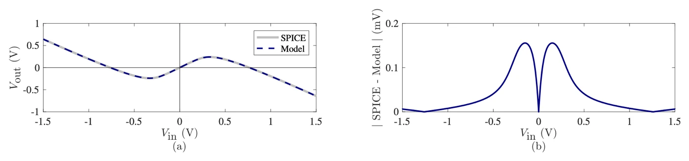
Two classic wavefolders, one built from a pair of transistors and one from two diodes and an op-amp, both turn a wave back on itself once it passes about 0.3 V, and the paper writes each as an exact formula that stays within 1 mV of a circuit simulator.
Abstract
Wavefolders are a particular class of nonlinear waveshaping circuits, and a staple of the “West Coast” tradition of analog sound synthesis. In this paper, we present analyses of two popular wavefolding circuits—the Lockhart and Serge wavefolders—and show that they achieve a very similar audio effect. We digitally model the input–output relationship of both circuits using the Lambert-W function, and examine their time- and frequency-domain behavior. To ameliorate the issue of aliasing distortion introduced by the nonlinear nature of wavefolding, we propose the use of the first-order antiderivative method. This method allows us to implement the proposed digital models in real-time without having to resort to high oversampling factors. The practical synthesis usage of both circuits is discussed by considering the case of multiple wavefolder stages arranged in series.
The paper’s abstract, as published under CC BY 4.0.
Read along
Each step quotes the paper, says what it means in plain words, and gives you the circuit to play. The paper is open access under CC BY 4.0, so its words and figures appear as published.
- Step 1 · What wavefolding is (§1)
- Step 2 · The first circuit (§2, Figure 1a)
- Step 3 · The straight part (§2.1, equation 12)
- Step 4 · Where the fold comes from (§2.1, equations 13–21)
- Step 5 · The Lambert-W function (§2.2, equations 22–26)
- Step 6 · Model against SPICE (§2.3, Figures 2 and 3)
- Step 7 · A note through the folder, RL 10 kΩ against 50 kΩ (§2.3, Figure 4)
- Step 8 · The second circuit: a folding cell (§3, Figures 5–8)
- Step 9 · The two circuits are nearly the same (§3.1, Figure 9)
- Step 10 · Aliasing, and the antiderivative method (§4.2, equation 45, Figures 13–15)
- Step 11 · RL as a timbre control (§5.1, Figure 11)
- Step 12 · What it costs (§5.2, Table 5)
- Step 13 · Six folding cells in a row (§6, Figures 16–18)
- Step 14 · Four transistor folders in a row (§6, Figures 19–21)
- Step 15 · Conclusions (§7)
Step 1 · What wavefolding is (§1)
The paper says
"Wavefolding is a type of nonlinear waveshaping common in West Coast synthesis where portions of the input signal that exceed certain threshold are inverted or "folded back", hence the name of the effect." (§1)
In plain words
A clipper flattens the top of a wave once it gets too big. A folder turns it round instead. Past a threshold, the wave heads back down, as if it hit a mirror. Push harder and it can pass through zero and keep going the other way.
Every turn puts extra bends into each cycle, and extra bends are extra harmonics. So as you push a note harder into a folder, the pitch stays put but the tone grows brighter and changes character. In the transistor folder below, at its middle setting, a sine under about 0.25 V comes out as a clean copy. Above that, the tops turn over.
Try it
The transistor folder from step 2, playing a sine. Its parts list is in step 2.
circuit FirstFolder setting input: 1 V, from 0.1 V to 1.2 V setting output: 0.66 V, from 0.1 V to 2 V setting load: 10k, from 1k to 50k V1 vcc gnd 15V V2 gnd vee 15V Q1 c in e1 2N3906 R1 vcc e1 15k Q2 c in e2 2N3904 R2 e2 vee 15k RL c gnd load U2 c f f opamp Ri f m 10k Rf out m 10k U1 gnd m out opampendPress Play to see the wave after the circuit, at out.
Turn input slowly up from 0.1 V and watch the Scope. Below about 0.25 V the wave stays smooth. Then its tops dip in the middle, and the dip deepens as you keep turning.
Step 2 · The first circuit (§2, Figure 1a)
The paper says
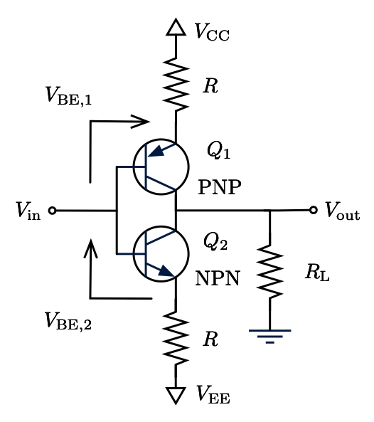
"The Lockhart wavefolder consists of an NPN and a PNP bipolar junction transistors connected at their base and collector terminals." (§2.1)
In plain words
Two transistors of opposite types, one PNP and one NPN, share the input at their bases and the output at their collectors. Each emitter hangs from a supply rail through 15 kΩ: the PNP's from +15 V, the NPN's from −15 V. The joined collectors drive a load resistor, RL, to ground. The paper tries RL from 1 kΩ to 50 kΩ (its Table 1), and RL turns out to be the circuit's main control.
The paper puts an inverting stage after it (§2.3), so the wave comes out the right way up. We add a follower in front of that stage, so it draws no current from RL: the paper's analysis assumes nothing does. Here the PNP is a 2N3906 and the NPN a 2N3904. SynthMaker's version stays within 0.016 mV of ngspice, a standard circuit simulator, at RL 10 kΩ (0.157 mV at 50 kΩ), with the same transistor models.
Try it
circuit FirstFolder setting input: 1 V, from 0.1 V to 1.2 V setting output: 0.66 V, from 0.1 V to 2 V setting load: 10k, from 1k to 50k V1 vcc gnd 15V V2 gnd vee 15V Q1 c in e1 2N3906 R1 vcc e1 15k Q2 c in e2 2N3904 R2 e2 vee 15k RL c gnd load U2 c f f opamp Ri f m 10k Rf out m 10k U1 gnd m out opampendPress Play to see the wave after the circuit, at out.
load is RL. The input runs to 1.2 V, the paper's own range (§2.1). U2 is the follower, and U1 with Ri and Rf is the inverting stage (the op-amp's two rules explains both). Open it in SynthMaker to change the parts.
Step 3 · The straight part (§2.1, equation 12)
The paper says
"IE,1 − IE,2 = −(2/R) Vin" (§2.1, equation 12)
In plain words
For small inputs, both transistors conduct, and each emitter resistor carries a steady current from its rail. Raise the input and one resistor gets a little less voltage across it while the other gets a little more. One current falls, the other rises, and the difference between them, 2/R times the input, flows through RL.
So for small signals the circuit is just an amplifier with a gain of 2RL/R. At RL 10 kΩ that's 2 × 10 kΩ / 15 kΩ = 1.33. On the real parts we measured 1.31. Across the whole range it holds within 1.5–3.5%: 0.132 against 0.133 at RL 1 kΩ, and 6.43 against 6.67 at 50 kΩ. The higher the gain, the shorter this straight part: at 50 kΩ it ends at 0.09 V in.
Try it
circuit FirstFolder setting input: 1 V, from 0.1 V to 1.2 V setting output: 0.66 V, from 0.1 V to 2 V setting load: 10k, from 1k to 50k V1 vcc gnd 15V V2 gnd vee 15V Q1 c in e1 2N3906 R1 vcc e1 15k Q2 c in e2 2N3904 R2 e2 vee 15k RL c gnd load U2 c f f opamp Ri f m 10k Rf out m 10k U1 gnd m out opampendPress Play to see the wave after the circuit, at out.
At 0.1 V in and RL 10 kΩ, the output is a clean sine about 0.13 V tall: the input times 1.31. Turn load down to 1k and it shrinks to about a tenth of the input. Turn it up to 50k and even this small input is past the straight part's end, so the tops start to fold.
Step 4 · Where the fold comes from (§2.1, equations 13–21)
The paper says
"the collector diodes in the large-signal model are antiparallel. Therefore, we can make the further assumption that only one of them will conduct at a time depending on the polarity of Vin." (§2.1)
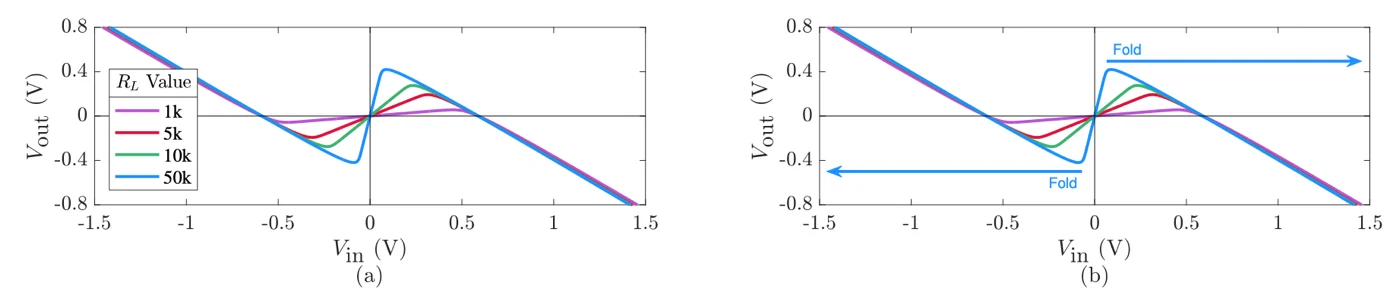
"increasing the value of RL sharpens the shape of the transfer function." (§2.3)
In plain words
Inside each transistor, the collector and the base meet at a junction, and a junction is a diode. The two collector diodes face opposite ways, so one can conduct on the positive half of the wave and the other on the negative half. While the output is small, both stay off. As it grows, the voltage across one of them grows too, until it reaches its knee and starts to conduct. Then it steals current that was going to RL, and the further the input goes, the more it steals. The output turns round: that's the fold. It's the same exponential knee that makes a diode clipper work, used to turn the wave back instead of flattening it.
RL decides where and how sharply. A bigger RL means more gain, so the output reaches the knee with a smaller input, and the turn is sharper. On the real parts, the turn moves from 0.45 V in at RL 1 kΩ to 0.09 V at 50 kΩ, and the output at the turn grows from 0.06 V to 0.42 V.
Try it
circuit FirstFolder setting input: 1 V, from 0.1 V to 1.2 V setting output: 0.66 V, from 0.1 V to 2 V setting load: 10k, from 1k to 50k V1 vcc gnd 15V V2 gnd vee 15V Q1 c in e1 2N3906 R1 vcc e1 15k Q2 c in e2 2N3904 R2 e2 vee 15k RL c gnd load U2 c f f opamp Ri f m 10k Rf out m 10k U1 gnd m out opampendPress Play to see the wave after the circuit, at out.
With input at 1 V, sweep load from 1k to 50k. At 1k the fold is soft and rounded, and the tone mellow. Towards 50k the corners sharpen and the sound turns buzzy.
Step 5 · The Lambert-W function (§2.2, equations 22–26)
The paper says
"Equation (21) describes an implicit relationship between the input and output voltages of the circuit; it cannot be solved algebraically. Instead, a closed-form solution for Vout can be derived with the help of the Lambert-W function." (§2.2)
In plain words
The paper's equation 21 has the output in it twice: once plainly, and once inside the diode's exponential. No amount of rearranging gets the output on its own. A circuit simulator handles that by guessing and correcting, over and over, until the numbers agree.
The Lambert W function is the named answer to exactly this kind of equation: W(x) is the number w for which w × e^w = x. With it, the paper writes the output straight from the input (equation 28): the straight part from step 3, minus a W term that stays near zero for small inputs and takes over at the fold. W itself is computed with a short, fixed iteration, the same small sum every sample with no open-ended searching, which is what a real-time model wants. The paper evaluates W with Fritsch's iteration (§4.1, equations 41–44). Our code module uses a simpler one: Newton's method on w + ln w = L, four steps from safe starting guesses (step 10 shows the code).
Is the formula right? We checked it against ngspice with the paper's own idealised transistors: within 0.8 mV, across the whole curve.
Try it
circuit FirstFolder setting input: 1 V, from 0.1 V to 1.2 V setting output: 0.66 V, from 0.1 V to 2 V setting load: 10k, from 1k to 50k V1 vcc gnd 15V V2 gnd vee 15V Q1 c in e1 2N3906 R1 vcc e1 15k Q2 c in e2 2N3904 R2 e2 vee 15k RL c gnd load U2 c f f opamp Ri f m 10k Rf out m 10k U1 gnd m out opampendA code module: its code is the whole of it, so there is no schematic.
Press Play to see the wave after the circuit, at out.
Switch between the circuit and the formula. The shapes are close but not the same: the formula folds a little later and higher, because it uses the paper's idealised transistors. Step 6 explains the difference. The formula's code is in step 10.
Step 6 · Model against SPICE (§2.3, Figures 2 and 3)
The paper says
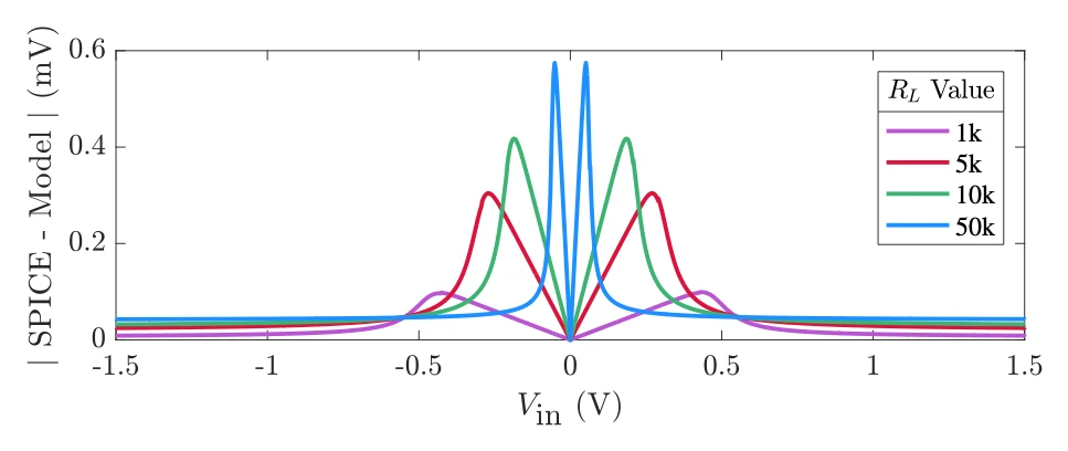
"the difference between the curves is indeed very small, below 1 mV for all values of Vin measured." (§2.3)
In plain words
SPICE is the standard circuit simulator, the one others are checked against. The paper draws its formula over SPICE's curves and finds them within 1 mV. We checked twice. The paper's formula against ngspice, with the paper's own idealised transistors: within 0.6–0.8 mV, which reproduces their result. And SynthMaker's circuit against ngspice, with the same models of real 2N3904 and 2N3906 transistors: within 0.004–0.157 mV across RL 1 kΩ to 50 kΩ.
Here's the twist. The paper's transistors are idealised: perfect, identical junctions (Is 10⁻¹⁷ A, η 1). Models of real parts fold earlier and lower. At RL 10 kΩ, the output turns at 0.28 V, where the paper's ideal transistors reach 0.38 V. At 50 kΩ it's 0.42 V against 0.57 V. The straight part's gain, 2RL/R, still holds within 3.5%.
Real PNP and NPN transistors also aren't mirror images of each other, so the two halves of the wave don't fold quite alike. The output sits slightly off centre, by 8 mV at RL 10 kΩ and 39 mV at 50 kΩ, and with that comes a trace of even harmonics that a perfectly symmetrical folder wouldn't make. So the paper's curves are for idealised transistors. What you play on this page are models of real parts.
Try it
circuit FirstFolder setting input: 1 V, from 0.1 V to 1.2 V setting output: 0.66 V, from 0.1 V to 2 V setting load: 10k, from 1k to 50k V1 vcc gnd 15V V2 gnd vee 15V Q1 c in e1 2N3906 R1 vcc e1 15k Q2 c in e2 2N3904 R2 e2 vee 15k RL c gnd load U2 c f f opamp Ri f m 10k Rf out m 10k U1 gnd m out opampendPress Play to see the wave after the circuit, at out.
On "RL 50k", look at where the wave sits on the Scope: not quite centred, because the two transistors don't match. On "RL 10k" the shift is smaller, 8 mV against 39 mV.
Step 7 · A note through the folder, RL 10 kΩ against 50 kΩ (§2.3, Figure 4)
The paper says
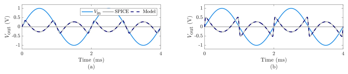
"For high values of RL the transition region between folded and non-folded values becomes very small and the resulting waveform is almost discontinuous (see Figure 4b). In the frequency domain, this will translate to higher harmonic content, similar to that of a square wave oscillator." (§2.3)
In plain words
Sharper folds make steeper edges, and steep edges are made of high harmonics. We sent a 500 Hz sine at 1 V through the real-parts circuit and measured the odd harmonics against the note itself. At RL 10 kΩ they fall away quickly: the 3rd at +1.3 dB, the 5th at −5.4 dB, the 7th at −11.6 dB and the 9th at −18.7 dB. At 50 kΩ they stay strong much higher up: the 3rd at +2.7 dB, the 5th at −2.2, the 7th at −5.6, the 9th at −8.3, the 11th at −10.5 and the 13th at −12.6 dB.
In both, the 3rd harmonic is louder than the note. At 50 kΩ even the 13th is only 12.6 dB below the note, where a square wave's 13th is 22 dB below its own. Measured against the note, its upper harmonics are stronger than a square wave's: that's the near-square buzz the paper describes.
Try it
circuit FirstFolder setting input: 1 V, from 0.1 V to 1.2 V setting output: 0.66 V, from 0.1 V to 2 V setting load: 10k, from 1k to 50k V1 vcc gnd 15V V2 gnd vee 15V Q1 c in e1 2N3906 R1 vcc e1 15k Q2 c in e2 2N3904 R2 e2 vee 15k RL c gnd load U2 c f f opamp Ri f m 10k Rf out m 10k U1 gnd m out opampendPress Play to see the wave after the circuit, at out.
Switch between the two. The pitch is the same; "RL 50k" is thinner, brighter and buzzier, and on the Scope its edges are nearly vertical. The buttons match the peaks, not the loudness.
Step 8 · The second circuit: a folding cell (§3, Figures 5–8)
The paper says
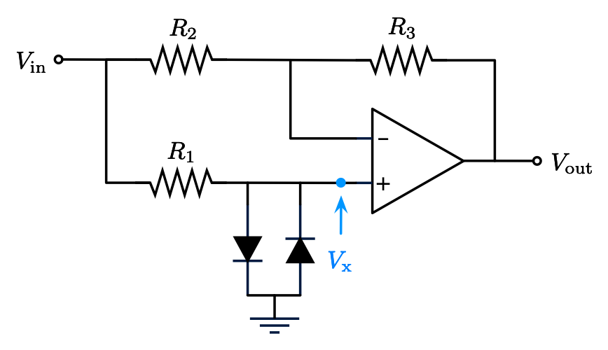
"Vout = 2Vx − Vin" (§3, equation 31)
"the circuit behaves as a wavefolder, folding portions of the input waveform whose absolute value exceeds approximately 0.3 V." (§3)
In plain words
The diode folder gets the same effect another way, from one op-amp, two diodes and three resistors. The input goes two ways. Through R1, 33 kΩ, it reaches node x, where two 1N4148 diodes facing opposite ways go to ground: a diode clipper. Through R2, 100 kΩ, it reaches the op-amp, which has R3, also 100 kΩ, as its feedback. With those two resistors equal, the op-amp's output is 2Vx − Vin: twice the clipped copy, minus the original.
While the diodes are off, x simply follows the input, so the output is 2Vin − Vin = Vin: a clean copy. Once the diodes hold x near their knee, x stops rising but the input doesn't, so the output falls: the fold. On SynthMaker's 1N4148 it turns at 0.331 V in, with 0.240 V out, close to the paper's "approximately 0.3 V". SynthMaker's cell is within 0.004 mV of ngspice. The paper's own formula for it (equation 39), whose diode values are the same 1N4148 values SynthMaker uses, is within 0.16 mV.
At 500 Hz and 1 V in, the cell has folded far enough that the note itself is quieter than its overtones: the 3rd harmonic is 12.0 dB louder than the note, the 5th 2.8 dB louder, then the 7th at −6.3 dB and the 9th at −18.0 dB. Our own diode wavefolder page builds three folds from op-amps and diode pairs, if you want to see the idea taken further.
Try it
circuit FoldCell setting input: 1 V, from 0.1 V to 1.2 V setting output: 0.66 V, from 0.1 V to 2 V R1 in x 33k D1 x gnd 1N4148 D2 gnd x 1N4148 U1 x m out opamp R2 in m 100k R3 out m 100kendPress Play to see the wave after the circuit, at out.
Turn input up from 0.1 V. At low input you get the sine back almost unchanged; past about 0.33 V, the tops fold down. Open it in SynthMaker and put a # in front of D1's and D2's lines: with no diodes, x just follows the input and the output never folds.
Step 9 · The two circuits are nearly the same (§3.1, Figure 9)
The paper says
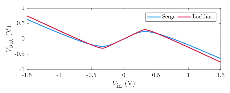
"the only significant difference between both transfer functions is in their sharpness at the folding points. This means the Lockhart wavefolder will introduce sharper folds which will translate into brighter sounds at the output." (§3.1)
In plain words
Set the transistor folder's RL to 7.5 kΩ and its straight part has a gain of 2 × 7.5 kΩ / 15 kΩ = 1, the same as the cell's clean copy. Drawn together, the two curves nearly match. In SynthMaker, the transistor folder turns at 0.266 V in with 0.243 V out, and the cell at 0.331 V in with 0.240 V out: almost the same height, with the transistor folder turning sooner and more sharply. Sharper corners, brighter sound, as the paper says.
They part company at large inputs. At 1 V in, the transistor folder's wave has swung out to 0.385 V, the cell's only to 0.240 V. So the two classic wavefolders, built from quite different parts, do nearly the same job, and the transistor one is a little brighter.
Try it
circuit FirstFolder setting input: 1 V, from 0.1 V to 1.2 V setting output: 0.66 V, from 0.1 V to 2 V setting load: 10k, from 1k to 50k V1 vcc gnd 15V V2 gnd vee 15V Q1 c in e1 2N3906 R1 vcc e1 15k Q2 c in e2 2N3904 R2 e2 vee 15k RL c gnd load U2 c f f opamp Ri f m 10k Rf out m 10k U1 gnd m out opampendPress Play to see the wave after the circuit, at out.
Switch back and forth at a few input levels. At low input they sound the same. As the folds arrive, the transistor folder is slightly brighter, and towards the top of the input knob they come apart. The buttons match the peaks at 1 V in, not the loudness.
Step 10 · Aliasing, and the antiderivative method (§4.2, equation 45, Figures 13–15)
The paper says
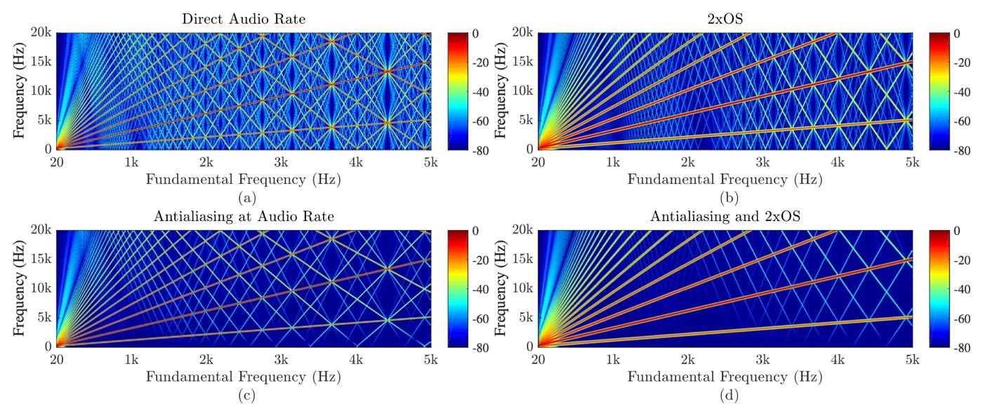
"Aliasing is known to cause unpleasant artifacts—such as beating and inharmonicity—that cannot be tolerated in a music computing scenario." (§4.2)
Vout[n] = (F(Vin[n]) − F(Vin[n−1])) / (Vin[n] − Vin[n−1]), "where F() is the antiderivative of f(), the original transfer function." (§4.2, equation 45)
In plain words
Digital audio at 48 kHz can only hold frequencies up to 24 kHz. A folder makes harmonics far above that. They can't simply vanish: they fold back down into the audible range at frequencies that have nothing to do with the note. Those are aliases, and they sound like faint, out-of-tune whistles and beating under the note, worst on high notes.
There are two cures. Oversampling runs the folder two or four times faster, so its harmonics have more room, then filters them before coming back down to 48 kHz. The antiderivative method, the paper's choice, changes the formula instead. Rather than reading the curve at each sample, it takes the curve's average between this sample and the last one, using its antiderivative F (the area under the curve): the change in area divided by the change in input, as equation 45 says. Averaging rounds off the sharp corners that make aliases.
We built the paper's formula (equation 28, RL 50 kΩ, its idealised transistors) as a code module and played a high note, about 1976 Hz, through each version in SynthMaker. Here's how loud the aliases are against the whole output, below 18 kHz:
| version | aliases |
|---|---|
| as written, 1× | −18.2 dB |
| oversampled 2× | −33.4 dB |
| oversampled 4× | −41.0 dB |
| antiderivative, 1× | −28.6 dB |
| antiderivative, 2× | −40.7 dB |
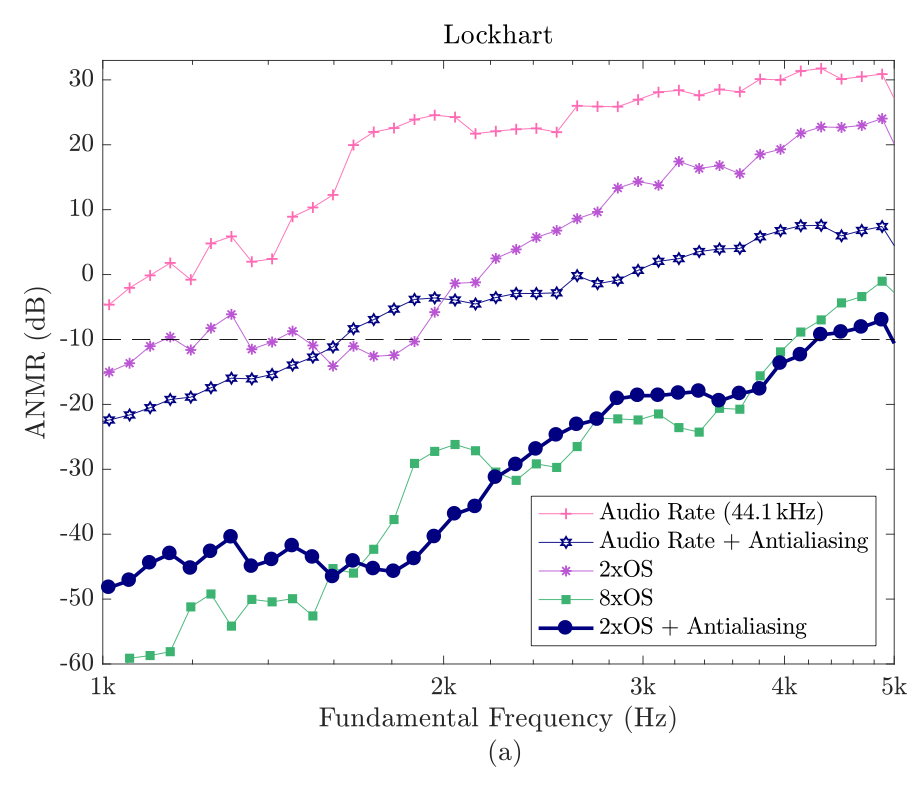
The antiderivative alone takes the aliases down 10 dB. At 2× it matches 4× oversampling, at half the sample rate. Measured on the formula outside the engine, with an ideal filter, it does even better: −53 dB against 4×'s −47 dB. The paper's own measure, ANMR, which weighs aliases by how audible they are, puts the antiderivative at 2× on a par with 8× oversampling.
Advanced: computing W. The paper uses Fritsch's iteration (§4.1, equations 41–44). Our module uses a simpler Newton iteration on w + ln w = L: one line for the starting guess, then four Newton steps, one line each. Newton's method converges safely here only from below the answer. The two starting guesses used, x/(1 + x) for small values and L − ln L for large ones, are both below it. A first try with a fixed guess of 0.5 gave NaNs (not-a-number results); the better guesses fixed it.
Try it
module FoldA2 in x out y oversample 2x lam = if x >= 0 then 1 else -1 L = -24.66926505792949 + lam * 296.42231157851324 * x ea = exp(min(L, 1.5)) wa0 = if L > 1.5 then L - log(max(L, 1.5)) else ea / (1 + ea) wa1 = wa0 - (wa0 + log(wa0) - L) / (1 + 1 / wa0) wa2 = wa1 - (wa1 + log(wa1) - L) / (1 + 1 / wa1) wa3 = wa2 - (wa2 + log(wa2) - L) / (1 + 1 / wa2) wa4 = wa3 - (wa3 + log(wa3) - L) / (1 + 1 / wa3) f = 6.666666666666667 * x - lam * 0.025864 * wa4 Fx = 3.3333333333333335 * x * x - 0.00004362694539130435 * wa4 * (wa4 + 2) y = (if abs(x - x') < 0.00001 then 0.5 * (f + f') else (Fx - Fx') / (x - x')) / 0.65endmodule Fold1 in x out y lam = if x >= 0 then 1 else -1 L = -24.66926505792949 + lam * 296.42231157851324 * x ea = exp(min(L, 1.5)) wa0 = if L > 1.5 then L - log(max(L, 1.5)) else ea / (1 + ea) wa1 = wa0 - (wa0 + log(wa0) - L) / (1 + 1 / wa0) wa2 = wa1 - (wa1 + log(wa1) - L) / (1 + 1 / wa1) wa3 = wa2 - (wa2 + log(wa2) - L) / (1 + 1 / wa2) wa4 = wa3 - (wa3 + log(wa3) - L) / (1 + 1 / wa3) f = 6.666666666666667 * x - lam * 0.025864 * wa4 y = f / 0.65endA code module: its code is the whole of it, so there is no schematic.
A code module: its code is the whole of it, so there is no schematic.
A code module: its code is the whole of it, so there is no schematic.
A code module: its code is the whole of it, so there is no schematic.
A code module: its code is the whole of it, so there is no schematic.
Press Play to see the wave after the circuit, at out.
This is the antiderivative version at 2×. f is equation 28; Fx is its antiderivative; the last line is equation 45, with x' meaning the previous sample's value (when two inputs are almost equal, it takes the average of f instead, to avoid dividing by nearly zero). The / 0.65 sets the level, like a circuit's output setting: 0.65 V of formula plays at full scale. "As written" drops the Fx line and ends with y = f / 0.65; the oversampled versions change only the oversample line.
Start on "As written, 1×" and listen under the note: there's a whistle of tones that don't belong to it. Step through the buttons. By "Oversampled 4×" and "Antiderivative, 2×" it's gone, and those two sound alike. Open it in SynthMaker to change the code.
Step 11 · RL as a timbre control (§5.1, Figure 11)
The paper says
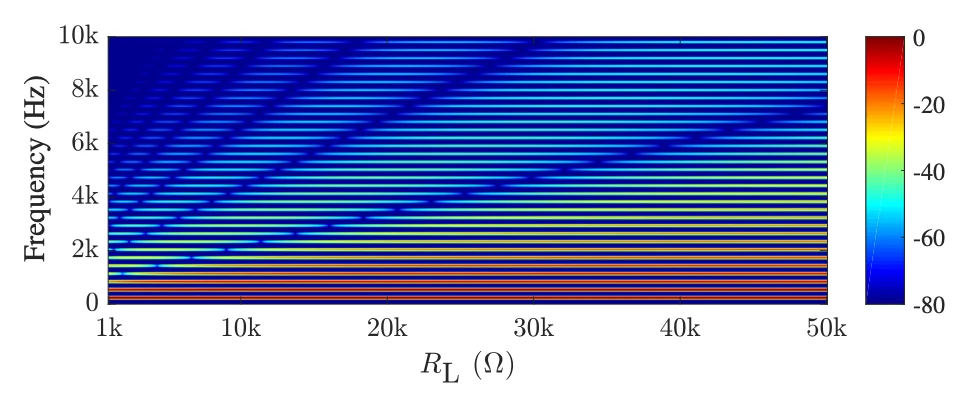
"the level of harmonic distortion introduced by the circuit is proportional to the value of this resistance. Therefore, this parameter can be used for additional timbral control." (§5.1)
In plain words
Steps 4 and 7 showed that a bigger RL folds sooner and sharper. That makes RL a tone control in its own right: turn it up and the sound gets brighter, without touching the input level. At 500 Hz and 1 V in, going from RL 10 kΩ to 50 kΩ lifts the 9th harmonic from −18.7 dB to −8.3 dB against the note, and brings the 13th up to −12.6 dB.
In SynthMaker the load is a setting, and a wire can turn a setting. Here a slow wave sweeps it, so you can hear the tone move on its own.
Try it
circuit FirstFolder setting input: 1 V, from 0.1 V to 1.2 V setting output: 0.66 V, from 0.1 V to 2 V setting load: 10k, from 1k to 50k V1 vcc gnd 15V V2 gnd vee 15V Q1 c in e1 2N3906 R1 vcc e1 15k Q2 c in e2 2N3904 R2 e2 vee 15k RL c gnd load U2 c f f opamp Ri f m 10k Rf out m 10k U1 gnd m out opampendPress Play to see its frequencies after the circuit, at out.
Hold a note and watch the Analyzer. As the load sweeps up, the upper harmonics climb and the tone opens up, then they fall back as it sweeps down. It works rather like a filter sweep, but by adding harmonics instead of removing them.
Step 12 · What it costs (§5.2, Table 5)
The paper says
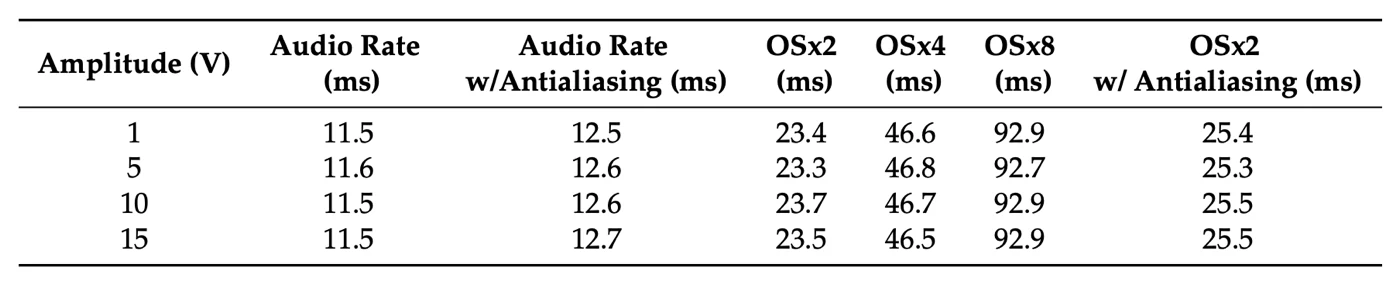
"the antialiased Lockhart model, implemented at a sample rate Fs = 88.2 kHz, is approximately 3.5 times faster than oversampling by a factor of 8" (§5.2)
In plain words
The paper's point is that its antialiased formula at twice the sample rate does the job of heavy oversampling for much less work: about 3.5 times faster than 8× oversampling.
What runs in the other steps here is different: not the formula, but the circuit itself, with models of real transistors, solved every sample. On our test machine it takes 371 ns per voice per sample at 1×, 668 ns at 2× and 1,243 ns at 4×. That's 1.8%, 3.2% and 6.0% of one processor core per voice. Each doubling of the rate costs a little under twice as much. So a chord of eight voices at 2× takes about a quarter of one core. The formula as a code module is far cheaper: well under 1% of a core per voice, even at 4×.
So the two aren't a like-for-like comparison. The formula is the fast route when you only need this one curve; the circuit is the route that lets you change any part and still hear what the real thing would do.
Try it
circuit FirstFolder oversample 1x setting input: 1 V, from 0.1 V to 1.2 V setting output: 0.66 V, from 0.1 V to 2 V setting load: 10k, from 1k to 50k V1 vcc gnd 15V V2 gnd vee 15V Q1 c in e1 2N3906 R1 vcc e1 15k Q2 c in e2 2N3904 R2 e2 vee 15k RL c gnd load U2 c f f opamp Ri f m 10k Rf out m 10k U1 gnd m out opampendPress Play to see the wave after the circuit, at out.
This is what the extra cost gets you, on the circuit itself. At 1×, a high note through the sharpest setting has aliases at −16.1 dB below 18 kHz. At 2× they're down to −40.4 dB, and at 4× to −51.7 dB. Listen under the note at 1×, then at 2×: most of the whistle is gone for less than twice the work.
Step 13 · Six folding cells in a row (§6, Figures 16–18)
The paper says
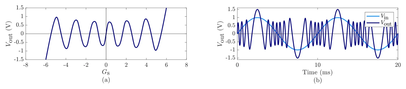
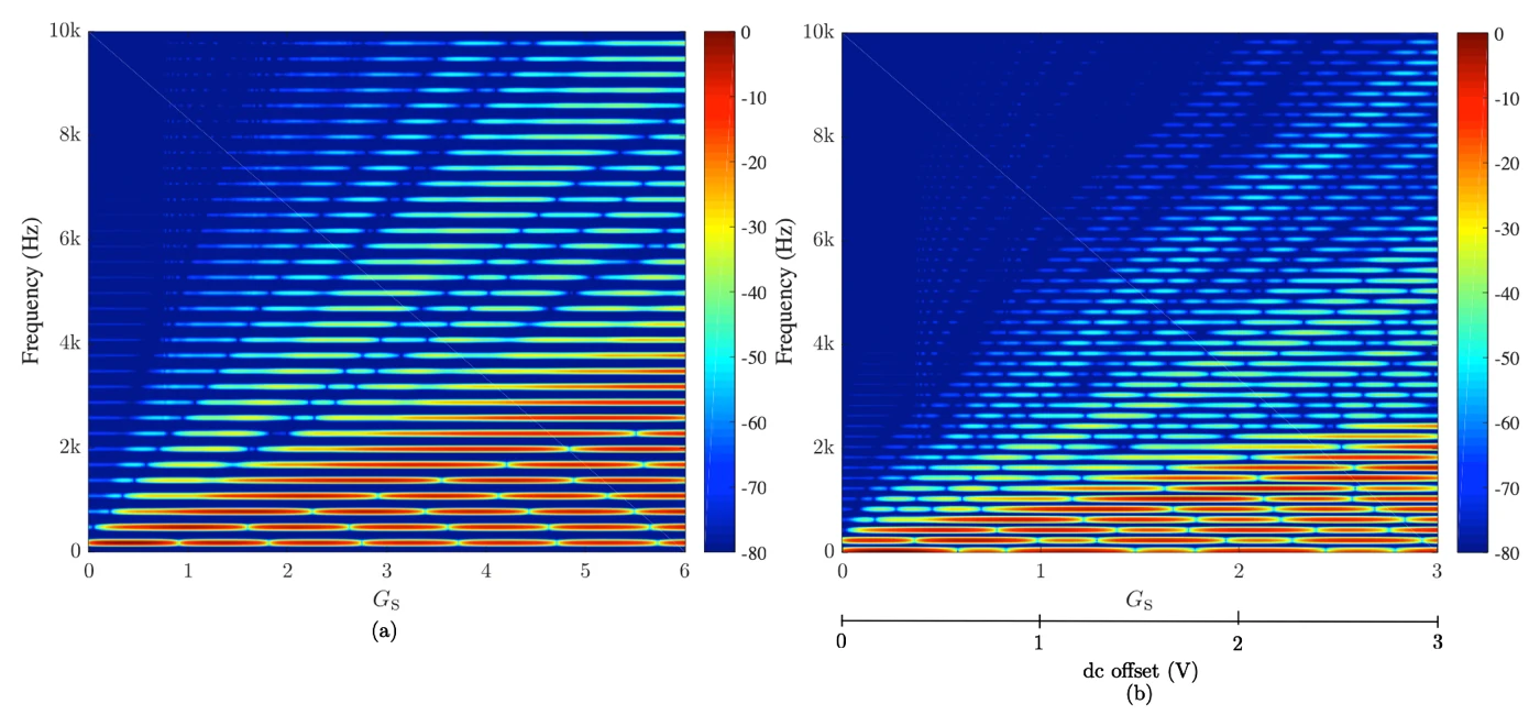
"In practical sound synthesis applications, a single folding stage is rarely used, as the timbral variety it can produce is quite limited." (§6)
"This parameter controls the amount of folds introduced, allowing the overall brightness of the sound to be varied. It can be modulated in real-time to provide articulation to a sound similar to filtering in subtractive synthesis or modulation index in FM synthesis." (§6)

In plain words
One cell from step 8 folds once each way. The full diode folder chains six of them, each feeding the next, with a gain stage, GS, in front. The more gain, the further the wave is pushed through the cells, and the more folds it collects. Measured in SynthMaker, with inputs up to 1 V, the curve turns 2 times at a gain of 2, 5 times at a gain of 4 and 6 times at a gain of 6. The output stays within 0.38 V either way all the while. The gain is "this parameter" in the quote: put an envelope on it and the brightness follows each note, much as a filter envelope does.
The six cells play here as two circuits of three, one after the other. That split changes nothing. The cells meet at op-amp outputs, and an op-amp's output holds its voltage while it drives the next cell, so cutting the circuit there is exact. We ran it both ways: as one circuit of six cells and as two circuits of three, the outputs agree within 0.00000012 V (1.2 × 10⁻⁷ V). The split version is cheaper too, 564 ns per sample against 837 ns at 1×, since smaller circuits are quicker to solve. That's how SynthMaker can run circuits too big for one circuit: split them where nothing loads the signal, and chain the pieces.
Try it
circuit CascadeA setting input: 1 V, from 0.1 V to 1 V setting output: 1 V Ug in g g0 opamp Rg1 g0 g 10k Rg2 g gnd 3.33333k R11 g0 x1 33k D1a x1 gnd 1N4148 D1b gnd x1 1N4148 U1 x1 m1 o1 opamp R21 g0 m1 100k R31 o1 m1 100k R12 o1 x2 33k D2a x2 gnd 1N4148 D2b gnd x2 1N4148 U2 x2 m2 o2 opamp R22 o1 m2 100k R32 o2 m2 100k R13 o2 x3 33k D3a x3 gnd 1N4148 D3b gnd x3 1N4148 U3 x3 m3 out opamp R23 o2 m3 100k R33 out m3 100kendcircuit CascadeB setting input: 1 V setting output: 0.43 V, from 0.1 V to 2 V R14 in x4 33k D4a x4 gnd 1N4148 D4b gnd x4 1N4148 U4 x4 m4 o4 opamp R24 in m4 100k R34 o4 m4 100k R15 o4 x5 33k D5a x5 gnd 1N4148 D5b gnd x5 1N4148 U5 x5 m5 o5 opamp R25 o4 m5 100k R35 o5 m5 100k R16 o5 x6 33k D6a x6 gnd 1N4148 D6b gnd x6 1N4148 U6 x6 m6 out opamp R26 o5 m6 100k R36 out m6 100kendPress Play to see the wave after the circuit, at out.
Ug, Rg1 and Rg2 are the gain stage: its gain is 1 + Rg1/Rg2, so 10k gives 2, 3.33333k gives 4 and 2k gives 6. Then come three cells in each circuit, each the cell from step 8. Step through the gains with input at 1 V and watch the wave gain more wiggles per cycle, then turn input down and hear the folds peel away one by one. Open it in SynthMaker to change the parts.
Step 14 · Four transistor folders in a row (§6, Figures 19–21)
The paper says
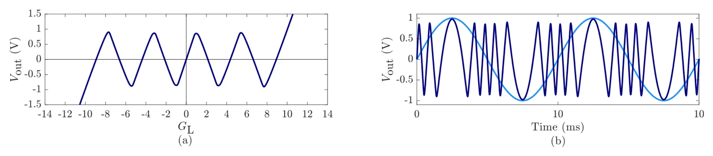
"Firstly, the individual folders must provide approximately unity gain for small input values, i.e., below the folding point, and approximately negative unity gain beyond the folding point. Secondly, each stage should start folding at the same point with respect to its individual input." (§6)
"In Section 3.1, it was shown that for RL = 7.5 kΩ the Lockhart wavefolder exhibits approximately unity gain below the folding point. This value leads to pre- and post-gains of approximately 1/3 and 3, respectively." (§6)

In plain words
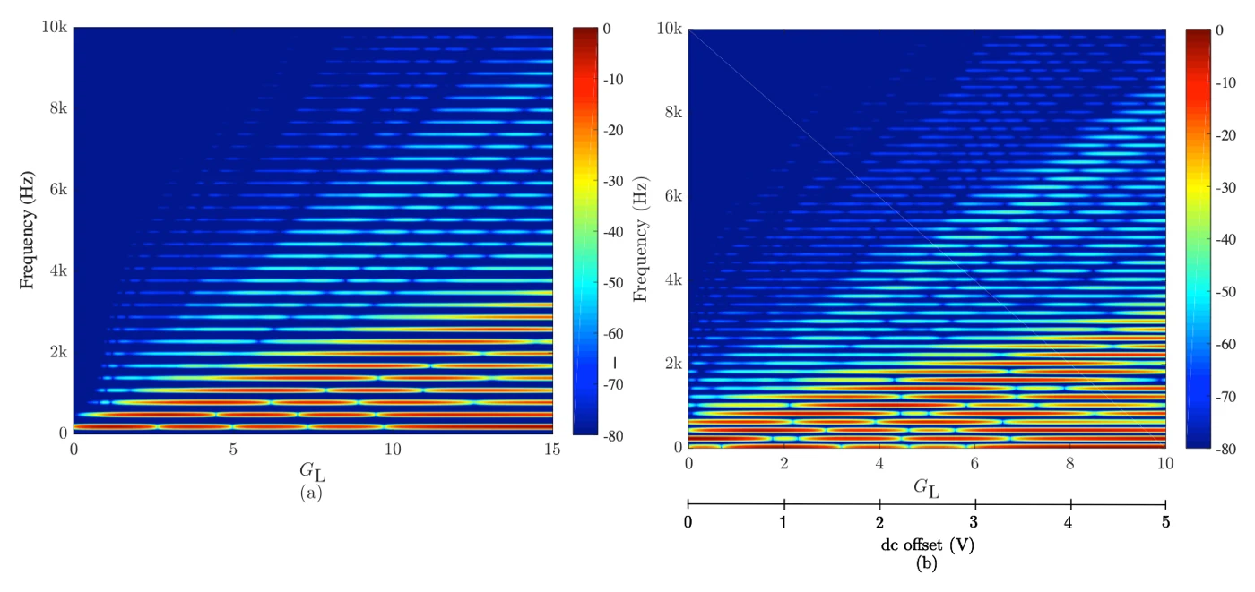
The transistor folder can be chained too, as long as each stage behaves alike: a gain of about 1 before its fold, about −1 after it, and the fold in the same place for each. Step 9 showed that RL 7.5 kΩ gives a gain of 1, so the paper uses that for all four stages. A gain of GL × 1/3 goes in front and × 3 after. Then come two optional extras the paper adds: a soft tanh curve, "to model the behavior of an output buffering stage and to limit the range of the output waveform", and a gentle low-pass at 1.3 kHz, "a simple tone control" (both §6).
As with the diode cells, GL sets how many folds you get. Measured in SynthMaker with real transistors, with inputs up to 1 V, the curve turns 2 times at GL 3, 3 times at GL 6 and 4 times at GL 10. And as in step 13, the chain plays as two circuits of two stages, joined at an op-amp's output. One circuit or two, the outputs agree within 0.00000024 V (2.4 × 10⁻⁷ V), and the split is cheaper: 1,401 ns per sample against 2,250 ns at GL 10.
Here's the twist. The paper says "The static gain blocks ensure the amplitude of the folded output is bounded between approximately ±1 V for values of GL between −10 and 10" (§6). With real transistors, that holds at GL 3 and 6, where the output stays between −0.77 V and +0.71 V. At GL 10 it doesn't: the output reaches +1.76 V. Real stages aren't exactly unity gain below the fold (step 3 found 2RL/R true only within 1.5–3.5%), and four stages in a row multiply the small differences. The tanh after the chain is what brings it back in range, which is the paper's own reason for it.
Try it
circuit ChainA setting input: 1 V, from 0.1 V to 1 V setting output: 1 V V1 vcc gnd 15V V2 gnd vee 15V Rg1 in mg 30k Rg2 g1 mg 60k Ug1 gnd mg g1 opamp Rg3 g1 mg2 10k Rg4 g0 mg2 10k Ug2 gnd mg2 g0 opamp Q1a c1 g0 e1a 2N3906 R1a vcc e1a 15k Q1b c1 g0 e1b 2N3904 R1b e1b vee 15k RL1 c1 gnd 7.5k U1f c1 f1 f1 opamp Ri1 f1 m1 10k Rf1 s1 m1 10k U1i gnd m1 s1 opamp Q2a c2 s1 e2a 2N3906 R2a vcc e2a 15k Q2b c2 s1 e2b 2N3904 R2b e2b vee 15k RL2 c2 gnd 7.5k U2f c2 f2 f2 opamp Ri2 f2 m2 10k Rf2 out m2 10k U2i gnd m2 out opampendcircuit ChainB setting input: 1 V setting output: 1 V V1 vcc gnd 15V V2 gnd vee 15V Q3a c3 in e3a 2N3906 R3a vcc e3a 15k Q3b c3 in e3b 2N3904 R3b e3b vee 15k RL3 c3 gnd 7.5k U3f c3 f3 f3 opamp Ri3 f3 m3 10k Rf3 s3 m3 10k U3i gnd m3 s3 opamp Q4a c4 s3 e4a 2N3906 R4a vcc e4a 15k Q4b c4 s3 e4b 2N3904 R4b e4b vee 15k RL4 c4 gnd 7.5k U4f c4 f4 f4 opamp Ri4 f4 m4 10k Rf4 s4 m4 10k U4i gnd m4 s4 opamp Rp1 s4 mp 10k Rp2 p1 mp 30k Up1 gnd mp p1 opamp Rp3 p1 mp2 10k Rp4 out mp2 10k Up2 gnd mp2 out opampendmodule Tanh in x out y # tanh(x), from exp (e^2x − 1) / (e^2x + 1) e = exp(2 * clamp(x, -15, 15)) y = (e - 1) / (e + 1)endmodule LowPass in x out y # one pole at 1300 Hz, its coefficient from the rate a = 1 - exp(-2 * pi * 1300 / rate) y = y' + a * (x - y')endmodule Trim in x out y y = x * 0.94endPress Play to see the wave after the circuit, at out.
In ChainA, Ug1 with Rg1 and Rg2 gives a gain of Rg2/Rg1, upside down: 60k / 30k = 2, which is GL 6 × 1/3. Ug2 turns it the right way up. Then come two transistor folders, each step 2's circuit at RL 7.5 kΩ. ChainB holds the next two and the × 3 gain (30k / 10k, turned the right way up by Up2). Step through GL 3, 6 and 10 with input at 1 V: the wave collects more wiggles and the sound brightens. On GL 10 the tanh is doing real work, rounding off the tops that real transistors push past 1 V. Open it in SynthMaker to change the parts.
Step 15 · Conclusions (§7)
The paper says
"In addition to this, we observed that the behavior of both circuits is very similar, despite the fact that their designs are fundamentally different." (§7)
"Within the context of the Lockhart wavefolder, it was shown that the proposed antialiased model is perceptually free from the effects of aliasing distortion when implemented at a sampling rate of Fs = 88.2 kHz." (§7)
In plain words
Two circuits built from quite different parts, a pair of transistors and an op-amp with two diodes, fold a wave in nearly the same way. Each can be written as an exact formula with the Lambert W function. And the antiderivative method lets the transistor folder's formula run at twice the usual sample rate, 88.2 kHz, with no audible aliasing.
What SynthMaker adds: - Both circuits, from real parts. They run in SynthMaker from parts lists, within 0.004–0.16 mV of ngspice with the same part models. - The formulas, checked. The paper's formulas match ngspice within 0.16–0.8 mV for the parts they assume, and real transistors fold earlier and lower (step 6). - The antiderivative method, heard. In our engine it does what the paper promises: at 2× it matches 4× oversampling (step 10). - Big chains, split exactly. Cascades can be cut where op-amps meet with no change to the sound, which is how SynthMaker runs circuits bigger than one circuit holds (steps 13 and 14).
Try it
- The authors' own real-time demo and their Lambert-W code: the paper's companion page.
- Our course page builds a three-fold diode folder from scratch: How a wavefolder works: folding with diodes.
Words you'll meet
- Wavefolder
- a circuit that turns a wave back on itself once it passes a threshold, instead of flattening it.
- Fold
- the point where the output turns round. More folds per cycle means more harmonics and a brighter sound.
- Transfer function (transfer curve)
- the output plotted against the input. A folder's curve rises, turns and comes back down.
- Harmonics, odd and even
- the frequencies at whole-number multiples of the note. A folder whose two halves fold alike makes only odd ones (3rd, 5th, 7th…); any mismatch adds a trace of even ones.
- Load resistor (RL)
- the resistor the transistor folder's output drives. It sets the gain, 2RL/R, and so how soon and how sharply it folds.
- Ebers–Moll model
- the classic large-signal model of a transistor: two diodes, one for each junction, plus current sources linking them. Its collector diodes are what make the transistor folder fold.
- Op-amp
- an amplifier with huge gain, used with resistors to make exact gains, followers (a gain of 1 that draws no current) and inverters.
- Lambert W function
- W(x) is the number w for which w × e^w = x. It solves equations that mix a value with its own exponential, like a diode's.
- SPICE (ngspice)
- the standard circuit simulator, used as the reference to check models against.
- Aliasing
- in digital audio, harmonics above half the sample rate fold back down to wrong, out-of-tune frequencies.
- Oversampling
- running a process at two, four or more times the sample rate, then filtering, so fewer harmonics alias.
- Antiderivative antialiasing
- averaging a curve between one sample and the next, using its antiderivative (the area under it), so sharp corners alias less.
- ANMR
- the paper's measure of aliasing, weighted by how audible it is.
- Cascade
- stages in a row, each feeding the next.
What we left out, and how faithful the patches are
What the patches are. Every circuit on this page is a parts list that SynthMaker solves as a circuit, every sample. Against ngspice with the same part models, they're within 0.004–0.157 mV (the transistor folder) and 0.004 mV (the diode cell). Split into two circuits, the six cells and the four stages match the same circuit run whole within 1.2 × 10⁻⁷ V and 2.4 × 10⁻⁷ V.
Real parts, not idealised ones. The paper's analysis and formulas assume idealised transistors with perfect, identical junctions. Our circuits use models of real 2N3904 and 2N3906 transistors, so they fold earlier and lower (0.28 V against 0.38 V at RL 10 kΩ), sit slightly off centre (8 mV at 10 kΩ, 39 mV at 50 kΩ), and, chained four deep at GL 10, overshoot the paper's ±1 V. The diode cell's formula uses the same 1N4148 values as our part, so there the paper's formula and ngspice agree within 0.16 mV.
Small changes to the circuits. A follower sits before each transistor folder's inverting stage, so nothing loads RL, as the paper's analysis assumes. One SynthMaker circuit holds up to 8 diodes and 8 op-amps, so the six-cell cascade (12 diodes) plays as two circuits of three cells, and the four-stage chain (10 op-amps) as two circuits of two stages. Both splits are exact. The tanh and the low-pass after the four-stage chain are ordinary SynthMaker modules rather than circuits.
What we measured differently. The paper measures aliasing with ANMR, an audibility-weighted measure; we use a plainer one, the aliases' share of the output below 18 kHz. The paper times its formulas; we timed our circuit itself (step 12). Our antialiasing comparison uses the paper's formula at RL 50 kΩ only.
What we didn't reproduce. The paper's spectrograms (Figures 13 and 21), its ANMR curves (Figure 15) and its timings (Table 5) appear as the paper's own figures, not remade. The DC offset on the six-cell cascade (Figure 18b) and on the four-stage chain (Figure 21) isn't in the patches. Nor is the diode cell's formula as a code module, or an antialiased version of it.
Further reading
- The paper: F. Esqueda, H. Pöntynen, J. D. Parker and S. Bilbao, "Virtual Analog Models of the Lockhart and Serge Wavefolders", Applied Sciences 7(12):1328, 2017. doi:10.3390/app7121328 (open access, CC BY 4.0).
- Our course page on folding: How a wavefolder works: folding with diodes.
- The diode knee behind every fold: How a diode clipper works.
- The follower and the inverting stage: The op-amp's two rules: buffer, gain and a mixer.
- From the reading list: SPICE2, the simulator others are checked against; and the antialiasing method the paper uses for its digital models, in Parker, Zavalishin and Le Bivic 2016 and Bilbao, Esqueda, Parker and Välimäki 2017.
- The authors' real-time demo and Lambert-W code: the paper's companion page.
- The function in step 5: Wikipedia: Lambert W function.